TRI-DEP: A Trimodal Comparative Study for Depression Detection Using Speech, Text, and EEG

Mancini, Eleonora; Nurfirdausi, Annisaa Fitri; Torroni, Paolo

TRI-DEP: A Trimodal Comparative Study for Depression Detection Using Speech, Text, and EEG

Eleonora Mancini^*, Annisaa Fitri Nurfirdausi^*, Paolo Torroni

DISI, University of Bologna, Italy
[TBD]
^*Indicates Equal Contribution

Abstract

Depression is a widespread mental health disorder, yet its automatic detection remains challenging. Prior work has explored unimodal and multimodal approaches, with multimodal systems showing promise by leveraging complementary signals. However, existing studies are limited in scope, lack systematic comparisons of features, and suffer from inconsistent evaluation protocols. We address these gaps by systematically exploring feature representations and modeling strategies across EEG, together with speech and text. We evaluate handcrafted features versus pretrained embeddings, assess the effectiveness of different neural encoders, compare unimodal, bimodal, and trimodal configurations, and analyze fusion strategies with attention to the complementary role of EEG. Consistent subject-independent splits ensure reproducible benchmarking. Our results show that the combination of EEG enhances multimodal detection, pretrained embeddings outperform handcrafted features, and carefully designed trimodal models achieve state-of-the-art performance. Our work serves as a robust benchmark for future research in multimodal depression detection.

Baseline Works

In this study, we implemented from scratch two multimodal baselines for comparison, both combining EEG and audio signals on the MODMA dataset. Yousufi et al. (2024) used DenseNet-121 as a feature extractor, while Qayyum et al. (2023) applied Vision Transformer (ViT) models for generating EEG and audio spectrograms.

Data Preparation for Baseline Works

EEG preprocessing follows Yousufi et al. (2024), including a 0.4–45 Hz FIR bandpass filter, a 50 Hz notch filter, and average referencing. We selected 29 channels (FP2, FP1, Fz, F7, F3, F4, F8, FT7, FC3, FCz, FC4, FT8, C3, C4, T3, CP3, CPz, CP4, T4, TP7, P3, Pz, P4, TP8, T5, T6, O1, Oz, O2) for analysis. Since Qayyum et al. (2023) provide limited details, we applied the same preprocessing pipeline to both baselines for consistency. For audio pre-processing, since both studies generate audio spectrograms directly from the original sampling rate of 44 kHz, we assume that no additional preprocessing was performed on the speech signals prior to spectrogram extraction.

EEG and Speech Spectrogram Generation

Following Yousufi et al. (2024) and Qayyum et al. (2023), we generate STFT spectrograms for EEG and mel-spectrograms for audio using librosa. We apply n_fft=1024, hop_length=512, and n_mels=64 (for audio). The resulting spectrograms are saved as .png images for use with 2D models such as DenseNet-121 and ViT.

Data Splitting

We use stratified 5-fold cross-validation with subject-level splitting to prevent data leakage. In each fold, 10% of the training data is set aside for validation (using a fixed random seed), resulting in train, validation, and test splits that preserve class balance.

Methodology

EEG Preprocessing

EEG preprocessing follows two pipelines depending on the feature extraction method.

Pipeline 1: We select 29 depression-related EEG channels [FP2, FP1, Fz, F7, F3, F4, F8, FT7, FC3, FCz, FC4, FT8, C3, C4, T3, CP3, CPz, CP4, T4, TP7, P3, Pz, P4, TP8, T5, T6, O1, Oz, O2]. Signals are bandpass filtered (0.5–50 Hz), notch filtered at 50 Hz, re-referenced to the average electrode, and segmented into 10-second windows.

Pipeline 2: We replicated the preprocessing steps of the CBraMod model for the MUMTAZ depression dataset. Signals are resampled to 200 Hz, bandpass filtered between 0.3–75 Hz, and notch filtered at 50 Hz. 19 channels are selected [FP2, FP1, F7, F3, F4, F8, FCz, C3, C4, T3, CPz, T4, P3, Pz, P4, T5, T6, O1, O2]. The signals are segmented into 5-second windows (1000 samples each at 200 Hz). Each recording is divided into multiple fixed-length windows, and each window is further split into 5 non-overlapping patches of 200 samples each.

Experiments and Results

Data Splitting

We perform all experiments at the subject level using stratified 5-fold cross-validation to preserve class balance. The same subject-level splits are used across experiments, ensuring reproducibility, fair comparability, and robust results reported as mean and standard deviation across folds.

Subject split configurations for stratified 5-fold cross-validation

Split	Fold 1	Fold 2	Fold 3	Fold 4	Fold 5
Train	`02010024, 02030006, 02030002, 02020008, 02010005, 02030017, 02030007, 02010025, 02020023, 02030009, 02020010, 02010036, 02020014, 02010018, 02020025, 02010022, 02030004, 02020021, 02010006, 02020015, 02010010, 02030005, 02010023, 02020026, 02010008, 02010012, 02020018`	`02010024, 02030006, 02020027, 02020010, 02010002, 02030017, 02030009, 02010025, 02020023, 02030014, 02020014, 02010034, 02020015, 02010013, 02020025, 02010015, 02030004, 02020021, 02010004, 02010012, 02010008, 02030005, 02010018, 02020026, 02010006, 02010011, 02020019`	`02020008, 02030005, 02010002, 02030006, 02010006, 02030002, 02010010, 02010006, 02010025, 02010012, 02020027, 02030007, 02020019, 02010022, 02020026, 02010018, 02010034, 02010023, 02010005, 02030017, 02010004, 02010001, 02010002, 02010025, 02010012, 02010008, 02010004`	`02020008, 02030009, 02010007, 02010006, 02010008, 02030002, 02010022, 02030014, 02010011, 02010036, 02030006, 02030004, 02010018, 02010022, 02010013, 02010025, 02020023, 02010002, 02030007, 02010024, 02010005, 02010015, 02010021, 02010001, 02010002, 02010004, 02010015`	`02020008, 02030007, 02010008, 02010014, 02010018, 02030006, 02010024, 02010025, 02010022, 02020027, 02010018, 02010022, 02010016, 02030004, 02010002, 02010010, 02030001, 02010003, 02010024, 02010025, 02010015`
Val	`02020016, 02010011, 02020022`	`02020016, 02020010, 02020022`	`02020016, 02020023, 02010008`	`02010010, 02020022, 02020018, 02010004`	`02010011, 02020019, 02020015, 02010004`
Test	`02010002, 02010004, 02010013, 02010034, 02020015, 02020019, 02020027, 02030014`	`02010005, 02010022, 02010023, 02010036, 02020008, 02020018, 02030002, 02030007`	`02010011, 02010015, 02010024, 02020014, 02020021, 02020022, 02020025, 02030009`	`02010008, 02010012, 02010025, 02020010, 02020016, 02020026, 02030005`	`02010006, 02010010, 02010018, 02020023, 02030004, 02030006, 02030017`
Training Labels	Healthy = 14, Depressed = 13	Healthy = 14, Depressed = 13	Healthy = 14, Depressed = 13	Healthy = 13, Depressed = 14	Healthy = 13, Depressed = 14

Baseline Results

Below, we present the results of the baseline models, along with the improvements obtained after hyperparameter tuning and the addition of the text modality.

Hyperparameter details for baseline works

Hyperparameters	ViT	DenseNet-121	ViT (After Tuning)	DenseNet-121 (After Tuning)
Learning Rate	0.0004	0.01	0.01	0.001
Optimizer	Adam	Adamax	Adam	Adamax
Epochs	70	30	70	40
Batch Size	100	16	100	32

Vision Transformer — Pooling strategies

Pooling	Accuracy	Precision	Recall	F1-Score
Attention	0.5321 ± 0.2028	0.5050 ± 0.2452	0.5183 ± 0.2026	0.4960 ± 0.2174
Max	0.5821 ± 0.1708	0.5550 ± 0.2274	0.5683 ± 0.1746	0.5495 ± 0.1964
AdaptiveAvg	0.5571 ± 0.2197	0.5267 ± 0.2592	0.5383 ± 0.2174	0.5189 ± 0.2345
GlobalAvg	0.5821 ± 0.2189	0.5533 ± 0.2619	0.5633 ± 0.2187	0.5494 ± 0.2356

DenseNet-121 — Pooling strategies

Pooling	Accuracy	Precision	Recall	F1-Score
Attention	0.4214 ± 0.1286	0.2876 ± 0.1161	0.3800 ± 0.1122	0.3238 ± 0.1080
Max	0.5000 ± 0.2414	0.4967 ± 0.2619	0.4833 ± 0.2276	0.4831 ± 0.2381
AdaptiveAvg	0.5036 ± 0.2601	0.3963 ± 0.2796	0.4583 ± 0.2472	0.4030 ± 0.2410
GlobalAvg	0.5536 ± 0.2583	0.5855 ± 0.2929	0.5417 ± 0.2486	0.5309 ± 0.2556

Vision Transformer — Before vs After manual tuning

Configuration	Accuracy	Precision	Recall	F1-Score
Qayyum et al., (ViT)	0.5821 ± 0.1708	0.5550 ± 0.2274	0.5683 ± 0.1746	0.5495 ± 0.1964
After manual tuning	0.6036 ± 0.1661	0.5867 ± 0.2327	0.5800 ± 0.1697	0.5597 ± 0.1897

Baseline Models — With / Without Text

Configuration	Accuracy	Precision	Recall	F1-Score
ViT	0.6036 ± 0.1661	0.5867 ± 0.2327	0.5800 ± 0.1697	0.5597 ± 0.1897
ViT + Text	0.6321 ± 0.2084	0.6133 ± 0.2711	0.6083 ± 0.2051	0.5966 ± 0.2324
DenseNet-121	0.6071 ± 0.2292	0.6100 ± 0.2768	0.5967 ± 0.2240	0.5856 ± 0.2399
DenseNet-121 + Text	0.6357 ± 0.2136	0.6367 ± 0.2630	0.6217 ± 0.2089	0.6089 ± 0.2278

Preliminary Studies

The framework supports various combinations of feature types, deep encoders, and late-fusion strategies. To structure the investigation and ensure feasibility, we first performed unimodal experiments for each modality (EEG, speech, and text) to identify the most effective model for each stream. These best-performing unimodal models were then integrated into the final multimodal pipeline. The result of preliminary studies can be seen below:

EEG Results

Model	Feature Group	Score
cbramod_conv	CBRaMod	0.4927 ± 0.1594
cbramod_mumtaz_conv	CBRaMod Mumtaz	0.4462 ± 0.1056
cbramod_mumtaz_lstm	CBRaMod Mumtaz	0.4424 ± 0.1019
xhand_cnn_fc	Handcrafted	0.4327 ± 0.1710
xhand_cnn_lstm	Handcrafted	0.4182 ± 0.0957
labram_gru_attn	LaBraM	0.4165 ± 0.0893
xhand_cnn_gru_attn	Handcrafted	0.4121 ± 0.1431
cbramod_mumtaz_gru_attn	CBRaMod Mumtaz	0.4038 ± 0.1386
cbramod_gru_attn	CBRaMod	0.3771 ± 0.1700
labram_lstm	LaBraM	0.3557 ± 0.0222
cbramod_lstm	CBRaMod	0.3501 ± 0.1557
labram_conv	LaBraM	0.2958 ± 0.0250

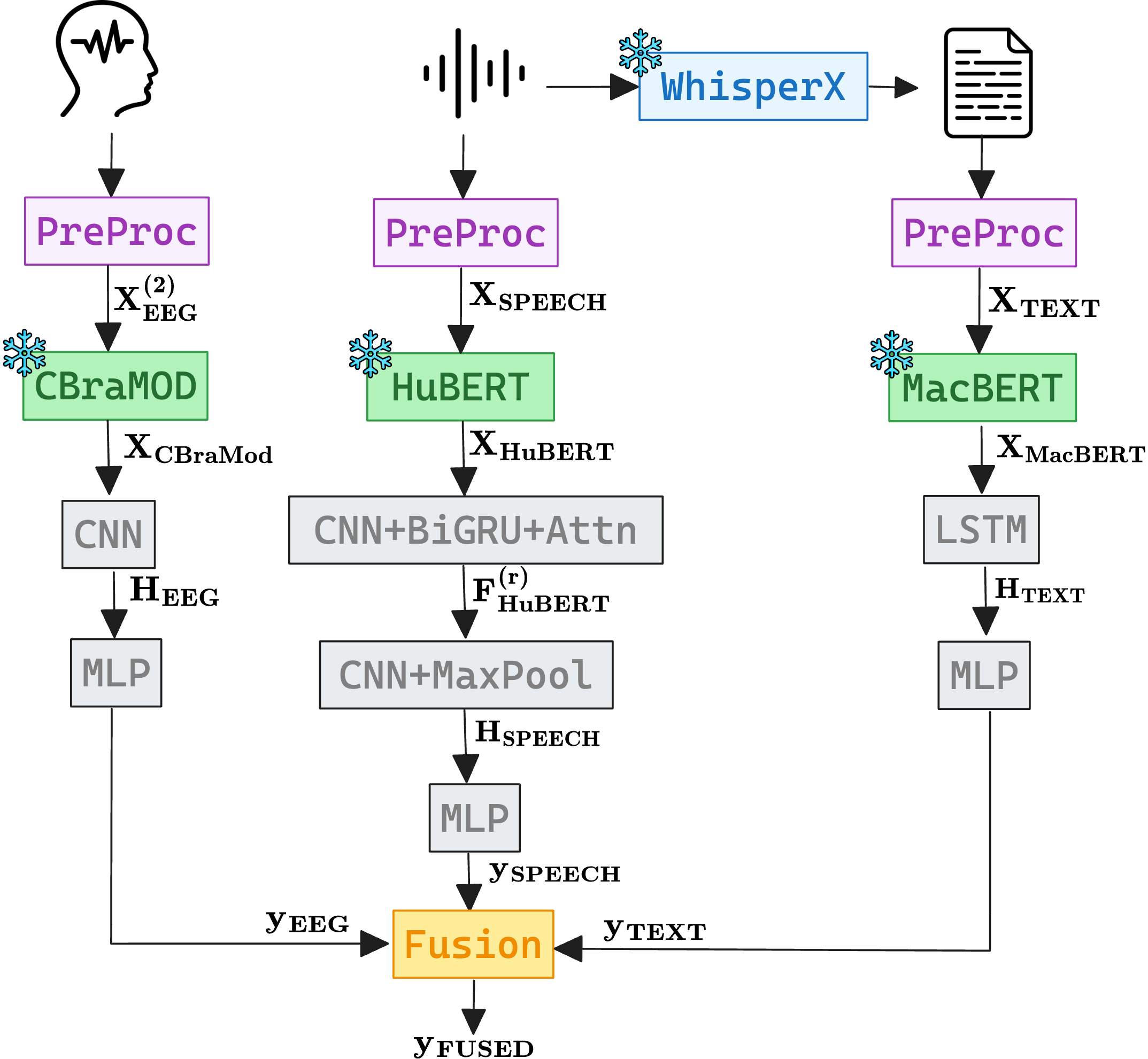
Best per feature group: CBRaMod cbramod_conv 0.4927 ± 0.1594; CBRaMod Mumtaz cbramod_mumtaz_conv 0.4462 ± 0.1056; Handcrafted xhand_cnn_fc 0.4327 ± 0.1710; LaBraM labram_gru_attn 0.4165 ± 0.0893.

Best overall EEG: cbramod_conv 0.4927 ± 0.1594.

Speech Results

Model	Feature Group	Score
hubert_bigru_conv	HuBERT	0.8090 ± 0.0812
hubert_noenc_lstm	HuBERT	0.8064 ± 0.0795
hubert_noenc_conv	HuBERT	0.7785 ± 0.0746
xlsr_cnn_conv	XLSR-53	0.7736 ± 0.1429
xlsr_cnn_lstm	XLSR-53	0.7474 ± 0.1594
xlsr_gru_lstm	XLSR-53	0.7261 ± 0.1344
hubert_bigru_lstm	HuBERT	0.7003 ± 0.1545
xlsr_lstm_conv	XLSR-53	0.6990 ± 0.2303
hubert_lstm_conv	HuBERT	0.6871 ± 0.0450
prosody_mfcc_bigru_attn	Prosody+MFCC	0.6549 ± 0.1820
xlsr_gru_conv	XLSR-53	0.6114 ± 0.2130
xlsr_lstm_lstm	XLSR-53	0.5805 ± 0.2201
mfcc_cnn_lstm	MFCC	0.5532 ± 0.1434
mfcc_lstm_conv	MFCC	0.5457 ± 0.1389
prosody_mfcc_cnn_lstm	Prosody+MFCC	0.5455 ± 0.1818
prosody_mfcc_cnn_bilstm	Prosody+MFCC	0.5455 ± 0.1818
mfcc_lstm_lstm	MFCC	0.4924 ± 0.1526
mfcc_bigru_conv	MFCC	0.4899 ± 0.2108
mfcc_bigru_lstm	MFCC	0.4555 ± 0.1395
mfcc_cnn_conv	MFCC	0.3846 ± 0.1453
hubert_lstm_lstm	HuBERT	0.3557 ± 0.0222

Best per feature group: HuBERT hubert_bigru_conv 0.8090 ± 0.0812; MFCC mfcc_cnn_lstm 0.5532 ± 0.1434; Prosody+MFCC prosody_mfcc_bigru_attn 0.6549 ± 0.1820; XLSR-53 xlsr_cnn_conv 0.7736 ± 0.1429.

Best overall Speech: hubert_bigru_conv 0.8090 ± 0.0812.

Text Results

Model	Feature Group	Score
macbert_lstm	MacBERT	0.7836 ± 0.1145
mpnet_lstm	MPNet	0.7684 ± 0.1485
mpnet_cnn	MPNet	0.7248 ± 0.2443
bert_cnn	BERT	0.7196 ± 0.1219
xlnet_lstm	XLNet	0.6655 ± 0.0876
bert_lstm	BERT	0.6460 ± 0.0849
macbert_cnn	MacBERT	0.6097 ± 0.1896
xlnet_cnn	XLNet	0.5638 ± 0.1723

Best per feature group: BERT bert_cnn 0.7196 ± 0.1219; MPNet mpnet_lstm 0.7684 ± 0.1485; MacBERT macbert_lstm 0.7836 ± 0.1145; XLNet xlnet_lstm 0.6655 ± 0.0876.

Best overall Text: macbert_lstm 0.7836 ± 0.1145.

Baseline and Multimodal Fusion Results (F1-score)

Category	Configuration	F1-score (mean ± std)
Baselines	ViT	0.560 ± 0.190
Baselines	DenseNet-121	0.586 ± 0.240
Weighted Averaging	EEG + Speech (0.05 : 0.95)	0.809 ± 0.081
	EEG + Text (0.15 : 0.85)	0.786 ± 0.116
	Speech + Text (0.45 : 0.55)	0.839 ± 0.059
	EEG + Speech + Text (0.05 : 0.35 : 0.60)	0.864 ± 0.095
Bayesian Fusion	EEG + Speech (0.05 : 0.95)	0.809 ± 0.081
	EEG + Text (0.05 : 0.95)	0.784 ± 0.114
	Speech + Text (0.20 : 0.80)	0.863 ± 0.140
	EEG + Speech + Text (0.05 : 0.30 : 0.65)	0.864 ± 0.095
Majority Voting	EEG + Speech	0.557 ± 0.135
	EEG + Text	0.500 ± 0.078
	Speech + Text	0.809 ± 0.081
	EEG + Speech + Text	0.800 ± 0.200

Table: Baseline and multimodal fusion results (F1-score, mean ± std across 5 folds). In bold, the best performing configuration per category; the overall best is additionally underlined. Fusion weights were optimized via grid search (step = 0.05).

Proposed Model

Based on our extensive experiments, we identified the best-performing models, and their overall architecture is illustrated below:

Illustration of best performing architectures observed — Best Architecture.